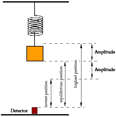
Figure 19-1: Schematic Diagram of the Apparatus
PROCEDURE
Setting Up the Apparatus
The basic set-up should have been
completed for you prior to lab, but you may need to make a few adjustments
before taking data. A schematic of the basic arrangement is illustrated
in Figure 19-1. The oscillating mass consists of standard masses
on a hanging mass holder suspended from the end of the spring.
Figure 19-1: Schematic Diagram of the Apparatus
The motion detector "sees" the bottom of the mass holder and reports this position to the DataLogger interface, and is analyzed by the LoggerPro application used earlier in the Motion experiments.
1. Before starting, check to see that the motion detector cable is connected to DIG/Sonic #1 of the interface box, and that the interface unit is turned on.
2. Click on the SHM.Link which opens the LoggerPro window. A graph with labeled axes should appear on your computer screen.
3. Suspend the spring WITHOUT MASSES, large end up, from the support hook, and position the motion detector on the floor directly under the spring. Do this by sighting through the spring from above to locate the appropriate position of the detector on the floor.
NOTE: This step needs to be done carefully so that the detector "sees" the mass clearly and without interference from, say, the edge of the table or other possible distractions.
NOTE: The motion detector must be shielded in case the mass accidentally falls. Be sure the detector is placed securely under the shield and is facing up.
4. Attach a mass to the spring. Use 150 grams to start (100 grams added to the 50-gram mass holder) and add additional weights only as needed. If you must, adjust the point of support so that the mass is not closer to the motion detector than about 0.75 meter.
5. Pull the mass straight down about 10 cm and then release it. Don't push it when you release it; try to release it cleanly.
6. After setting the mass in motion, click Collect in the LoggerPro window to begin data collection. Be sure the detector "sees" the mass over its full range of motion. There should be no flat portions to your graph. If there are, adjust scales, add mass, or reposition the detector and begin again. Some sources of error could be the detector "seeing" the bench or the clamp, so try to move it as far away from these items as is feasible.
7. Adjust the distance scale in the Graph Window so that the plot nearly fills the graph. To do this, double click anywhere on the graph to get a dialog box; then set the necessary maximum and minimum distance values.
8. When you are satisfied with your set-up and are ready to take actual data, open the Worksheet and fill in the header information. Then move on to the procedures below.
Activity #1: Making distance and velocity graphs.
The LoggerPro software automatically computes velocity and acceleration from the position information supplied by the interface unit. These data are stored in different files within the program each time a run is completed and also can be displayed graphically on the computer screen.
1. To display the graphs for distance and velocity, open the Distance-Velocity link.
2. Pull the mass straight down about 10 cm and then release it. Don't push it when you release it; try to release it cleanly.
3. After setting the mass in motion, click Collect in the LoggerPro window to begin data collection. Be sure the detector "sees" the mass over its full range of motion. There should be no flat portions to your graph. If there are, adjust scales, add mass, or reposition the detector and begin again. Some sources of error could be the detector "seeing" the bench or the clamp, so try to move it as far away from these items as is feasible.
4. Adjust the distance scale in the Velocity Graph Window so that the plot nearly fills the graph. To do this, double click anywhere on the graph to get a dialog box; then set the necessary maximum and minimum distance values.
5. When you are satisfied with your graphs, Copy and Paste them into the appropriate block on the Worksheet.
6. Answer the Questions 1 through 3 on the Worksheet about these graphs.
Activity #2: Properties of Periodic Motion
1. To measure the period and frequency of the motion represented by the graph, select Examine under the ANALYZE Menu in the LoggerPro Window. A vertical line with a cursor will appear. Drag this line to various points on the curve. Values for the x- and y-coordinates of the graph at the position of the cursor will appear in the information box.
2. Set the vertical line at the left-most peak of the distance graph. Record the time listed below the graph in cell E37 of the Worksheet.
3. Move the vertical line to the right, counting peaks as you go. Set the vertical line on the right-most peak. Record the time given below the graph in cell E38 of the Worksheet. Also record the number of cycles you counted in cell E39. The total time is the difference between these two time values, and the period of the motion is the total time divided by the number of cycles counted; that is, the period is the time for one cycle. The frequency is the number of cycles per second, which is the reciprocal of the period. The spreadsheet will do the calculations and display the results.
The midpoint of the motion is the point where the mass hangs when it is at rest. This position is the equilibrium position. The amplitude of the motion is the maximum displacement from the equilibrium position in either direction. For simple harmonic motion, the displacement from equilibrium should be the same in either direction.
4. Use ANALYZE...Examine with the cursor again to determine the closest distance and the farthest distance of the oscillating mass from the detector. Enter these values in cells E43 and E44 of the Worksheet.
The equilibrium position is midway between the closest and the farthest distances. The amplitude is the difference between either the farthest distance and the equilibrium distance, or the closest distance and the equilibrium distance. The spreadsheet will do the calculation and display the result.
Activity #3: Determining the force constant
1. With 150 grams suspended from the spring (50 grams for the carrier plus 100 grams), use the meter stick to carefully measure the equilibrium position of the mass when it is at rest. To do this, stabilize the mass as best you can, and measure the position of its bottom surface relative to the floor using the meter stick.
2. Transfer your data (in kg and meters) for both mass and position to cells B53 and C53 of the Worksheet.
3. Add a second 100-gram mass (so the total is now 250 grams) and measure the equilibrium position again. Transfer these data to cells B55 and C55 of the worksheet. Repeat with a third total mass of 350 grams, and enter the data in cells B57 and C57.
The force constant k is
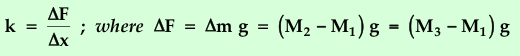
The original mass is M1 and the other two masses are M2 and M3, respectively.
4. The spreadsheet will automatically find the difference in force and the difference in mass, and perform the appropriate division with each pair of data points. The average value of k is displayed in cell F58.
Activity #4: Comparing distance, velocity and
acceleration graphs
1. To obtain a plot of the acceleration, open the Three-Graphs link.
2. Place a total of 200 grams (150 g plus 50 g holder) on the spring.
3. Start the mass oscillating with an amplitude of about 10 cm, and record this motion on the screen. Again, make sure the position curve is not "flat-topped".
4. Change the Time axis to display about three complete cycles, and adjust the Distance, Velocity and Acceleration scales until the graphs nearly fill the axes.
5. Answer Questions 4 through 11 on the Worksheet pertaining to these graphs.
Activity #5: Energy in SHM
1. First, select the bottom graph (Acceleration vs. Time) with the mouse so that "handles" appear. In LoggerPro, select MENU...Delete so that only plots of distance vs. time and velocity vs. time are displayed. Adjust scales so that about three complete cycles are shown.
2. Locate a point on the distance graph where the kinetic energy is zero, and use ANALYZE...Examine with the cursor to obtain a numerical value for this position.
3. Record the value of this distance in cell E84 under Point A on the Worksheet. Also enter the corresponding equilibrium distance for this situation in cell E85, by taking the one-half the sum of the peak and the valley distances off the plot. The equilibrium distance is just the average of the peak and valley distances.
4. The net elastic potential energy (EPE) of the spring at this point referenced to the equilibrium position is determined by:
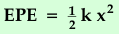
where x is the distance from the equilibrium position and k is the spring constant you measured earlier in this experiment. The value of the elastic potential energy is computed automatically by the spreadsheet and appears in cell E88.
5. Locate a point on the velocity graph where the net elastic potential energy is zero, and use ANALYZE...Examine with the cursor to obtain a numerical value for the velocity at this point.
6. Record the value of this velocity in cell E91 under Point B on the Worksheet.
7. Record the value of the hanging mass in cell E92.
In all of our problems, we assume that
the spring has zero mass. This simplifies the arithmetic but is clearly
not realistic in the laboratory. The spring has mass and is moving. And
one other complication exists: the bottom of the spring is moving with
the hanging mass, but the top is stationary at the point of support, and
the parts of the spring in between move with velocities in between these
values. We will account for this by introducing the idea of "effective"
mass of the spring representing some fraction of its total mass. But how
to determine the right fraction?
Recall that the period, spring constant, and mass are related in the following way:
T2 = 4π2M / k
or
M = T2k / 4π2
where M represents the sum of the hanging mass and the effective mass of the spring. Let m1 be the hanging mass and m2 be the effective spring mass. Then M = m1 + m2.
The measured values for T and k will be used to calculate M via the spreadsheet. The result appears in cell E95.
8. Now use M rather than the hanging mass to calculate kinetic energy. The Worksheet is set up to do this automatically. Assuming other values have been entered correctly, the answer will appear in cell E97.9. Now pick a point where the kinetic energy of the mass is not zero and the potential energy of the spring is not zero. Call this point C on your distance and velocity graphs, and enter the distance and equilibrium distance in cells E101:E102, as was done before in step 3. Enter the velocity in cell E106. The kinetic energy at C and the potential energy at C will be automatically calculated and the result displayed in cells E105 and E108. The Worksheet will transfer these values to a table which displays the EPE, KE and total energy at each of the three points A, B and C. Examine the results and answer Question 12 on the Worksheet.
10. Now measure the actual mass of your spring on the balance in the laboratory, and enter the result in cell E123.
The spreadsheet will use this real mass and the effective mass of the spring calculated above to compute the fraction m2 / mreal. The result will be displayed in cell E128.
11. Answer Question 13, print out the Worksheet, and submit it to your lab instructor.