| Average Velocity |
 |
|
| Instantaneous Velocity |
 |
PRELAB
PURPOSE
You will study how the average velocity approaches a fixed value as the time interval over which it is measured approaches zero.
EQUIPMENT air track, glider, two photogates, shims
RELEVANT EQUATIONS
| Average Velocity |
|
|
| Instantaneous Velocity |
|
DISCUSSION
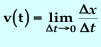
The concept of the instantaneous velocity as the limiting value of the average velocity taken over smaller and smaller time intervals is important in the study of motion. When the velocity is constant at all times, then the average value of the velocity, as defined in the first equation above will give the same value no matter how large or small the time interval is. However, if the velocity is changing from instant to instant, and we examine the average value centered about a specific time t, then the ratio of the distance covered Δx, divided by the time interval Δt, depends on the width of the time interval Δt over which the average is taken. It is an amazing consequence of the limiting process that if the time interval around time t is successively reduced, then the average velocity approaches a fixed limiting value. We can define this limiting value to be the instantaneous velocity at time t. The limiting process is illustrated in Figure 6-1, where the average velocity is seen to be the slope of the straight line connecting points A and B. As we squeeze down on the interval about time t, this slope, and thus the average velocity, approaches a fixed value.
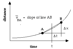
An air track provides a nearly frictionless surface for one-dimensional motion of a glider. If the track is level and the glider is given a slight nudge, it will move with constant velocity along the length of the track. Since the velocity is constant, the average velocity measured between any two points on the track is equal to the instantaneous velocity of the glider.
Figure 6-1: Air Track Set-up for Measurement of Instantaneous Velocity
Referring to Figure 6-1, if points A and B are selected, the average velocity is:
where: Δx is the distance from A to B and Δt is the time for the glider to move from A to B.
If the track is tilted slightly
so that the glider accelerates from A to B, the velocity
will be different at every point between A and B. The velocity
increases at a constant rate due to gravity as the glider moves toward
B.
The average velocity measured between A and B (![]() )
will be less than the instantaneous velocity at point B,
vB(t),
because the velocity is increasing as it moves towards point B.
)
will be less than the instantaneous velocity at point B,
vB(t),
because the velocity is increasing as it moves towards point B.
To experimentally estimate vB(t), you can use the definition of instantaneous velocity:
As you move A closer to B
many times, each new value of ![]() approximates vB(t), better, but it is still
less than vB(t). Since it may be impractical
to make Δx, and hence Δt, small enough for
approximates vB(t), better, but it is still
less than vB(t). Since it may be impractical
to make Δx, and hence Δt, small enough for
![]() to equal vB(t), you can extrapolate to
Δt = 0 on a graph of
to equal vB(t), you can extrapolate to
Δt = 0 on a graph of
![]() versus Δt
versus Δt
It may have already occurred to
you that a better estimate of vB(t) could
be made using points on each side of B (e.g. A and C
of Figure 6-1). Since the velocity is less than vB(t)
on the "A side" of B and greater than vB(t)
on the "C side" of B, ![]() should produce a better approximation to vB(t)
than the one sided procedure. You can move both C and A closer
to B and calculate new values of
should produce a better approximation to vB(t)
than the one sided procedure. You can move both C and A closer
to B and calculate new values of ![]() for successively smaller values of Δx and Δt.
These
for successively smaller values of Δx and Δt.
These ![]() values usually converge to vB(t)
faster than the
values usually converge to vB(t)
faster than the ![]() values. A graph of
values. A graph of ![]() versus Δ can still help you extrapolate to Δt =
0. You will use this three-point procedure to estimate an air track glider's
instantaneous velocity at a point B midway between measuring points
A and C.
versus Δ can still help you extrapolate to Δt =
0. You will use this three-point procedure to estimate an air track glider's
instantaneous velocity at a point B midway between measuring points
A and C.
Print out and complete the
Prelab questions.