1. Answer Question 1 on the Worksheet.
2. Use the spreadsheet calculator to determine the standard
deviation of the mean for the Δt data in part II.
a. The average Δt data that you computed in cells
B25:G25 has automatically been transferred
to cells B50:G50.
b. Select cell B51
as the location where the Standard Deviation for the Δx
= 120 cm run will be evaluated. Hit the Formula Builder
button  to
obtain the dialog box shown below.
to
obtain the dialog box shown below.
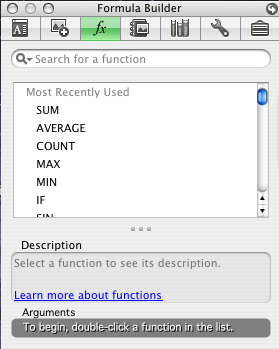
Under Statistical Functions, double click on STDEV.
You will see the screen below:
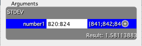
With the mouse, select cells B20:B24
to fill in the Number 1 line. Hit Return and the Standard
Deviation s, of the Δx
= 120 cm data set will appear in cell B51.
c. To find the Standard
Deviation of the Mean sm, the
Standard Deviation must be divided by the square root of the number of
data points. In cell B52, enter "=
B51/SQRT(5)".
d. You can now repeat the
same calculations for all the rest of the Δx
runs. The spreadsheet has a nice feature that automates this.
Select all the cells from B51 to G51 by dragging the mouse
across them. Under the EDIT menu, choose FILL....RIGHT.
The correct formulas will be automatically filled in using relative locations
for the cells.
e. Repeat for cells B52
to G52. Under the EDIT menu, choose FILL....RIGHT.
The Standard Deviation of the Mean for each data set appears.
3. Using the Δx and the average Δt
values for each run, compute the average velocity. In cell B54,
enter: "= 120/B50". Use the
EDIT...FILL....RIGHT feature to complete the calculation for all the
Δx runs in cells B54:G54.
4. Determine the uncertainty in each of the average velocities
Δv, calculated
above, and enter the values in cells B55:G55. Use the standard deviation
of the mean sm in Δt
for the uncertainty in Δt.
Do not forget the uncertainty in Δx.
Careful work should produce an uncertainty in Δx
of less than ±2 mm. The relative uncertainty in v
is equal to the sum of the relative uncertainties in Δt
and Δx, so the
entry in cell B55 should calculate Δv = v (Δt/t +
Δx/x)
In cell B55, enter: "= B54 * (B52/B50
+ 0.2/120)". Again use EDIT...FILL...RIGHT
to complete the results in cells B55:G55.
5. Make a graph of vavg versus Δt,
with Δt on the
horizontal axis, by using the Chart Wizard. Select the Δt
data in cells B50:G50, and, while holding down the apple button,
select the vavg
data by selecting cells B54:G54.
Select the x-y scatter icon
 from the top Toolbar.
Click on the chart itself.
Click on the legend and hit Delete.
From the View menu, select the Formatting Palette if it
is not already present.
Select Chart Title from the Title pull-down menu and
fill it in.
Next select titles for the Horizontal and Vertical
axes and fill them in.
6. Extrapolate
your graph to Δt = 0 to find the instantaneous velocity of the
glider at the 100 cm mark. Click on any one of the data points.
Choose Chart...Add Trendline from the menu.
Under the Options tab, choose Display
equation on chart. The equation of the best straight line fit to the
data will appear on the chart.
Use the mouse to size the chart and to locate it below the data.
Examine the fitting equation and enter the intercept in cell D57.
7. Estimate the uncertainty in the instantaneous velocity of the
glider and enter it in cell D58.
8. From the data of Part III, calculate the average
velocity, and enter the value in cell D65. Answer Question 2
in the space provided.