AND
ELECTRIC POTENTIAL
PROCEDURE
Parallel plates
Open up the Electric Workbook and fill in the header information. The field mapping apparatus consists of special graphite impregnated paper with metallic electrodes painted on it to simulate the distribution of electric charge that makes up the field source.
Take the parallel plate electrode sheet and note that there is a set of 1 cm X 1 cm grid squares printed on it as indicated by the crosses at each corner. The full sheet has a total of 29 marks along each horizontal row (counting the boundaries at 0 and 28), and 21 marks along each vertical column (counting the boundaries at 0 and 20).
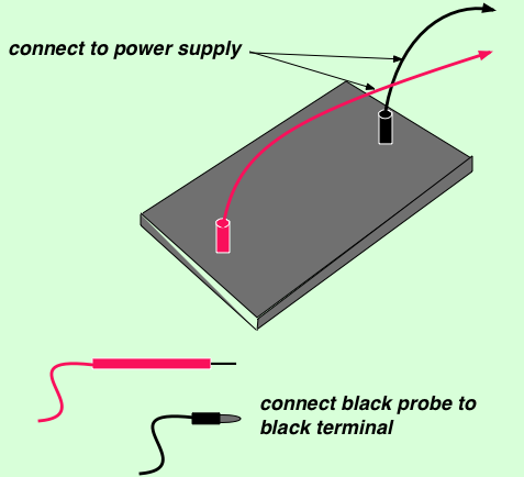
Mount the parallel plate electrode arrangement on the board provided. Connect the 30 V @ 1 A supply leads to make good contact with each electrode. Before switching the supply on make sure that the control knob is turned fully counter-clockwise. An illustration of the set up is shown below:
NOTE: If the electrical supply is provided through the distribution outlet on your bench, a knife switch has been supplied in the circuit. Please keep the switch open at all times when you are not making measurements.
Equipotential Measurements on
the Parallel Plate Configuration
1. Connect the digital voltmeter across the two electrodes on the board. Set the buttons to read volts on the 20 volt scale. Turn on the power supply and slowly increase the voltage knob until the voltmeter reads 5.0 volts. Record the voltage in cell M11. Disconnect the voltmeter.
2. Use an alligator clip to connect the black probe to the electrode that is connected to the negative power supply terminal. The red probe will be used to record the data at every other grid point on the paper. The data will consist of series of voltages taken along a specific column of grid points on the paper, that is each series will consist of 11 points, ranging from row 0 to row 20, by twos (e.g., 0, 2, 4, 6, ……, 20). The next series will be measured along column #2, and so forth, until 15 series of 11 data points are taken. See the outline plan in Figure 15-3 below.
Fig. 15-3: Grid Numbering Arrangement
4. Press Collect. Starting at the column at the extreme bottom-left of the grid sheet (row 0, column 0), place the red probe on the crosshair and after the voltage settles down, hit Keep. Do not be concerned about the time readout - it is irrelevant. Continue by placing the probe at row 2 and hitting Keep, then row 4, etc., all the way to row 20. Then hit Stop.
5. Select Table Window. The 11 points for column #0 should appear in the Table Window. With the mouse, select all of the Potential data and hit EDIT...COPY to save this data on the clipboard.
6. Select the Electric Workbook window, and EDIT...PASTE the data in the first column on the Spreadsheet where indicated.
7. Next, switch back to the field-plotter window, and repeat the same procedure for column #2, saving 11 data points in all. Perform the copy and paste routines to the Spreadsheet.
8. Repeat the same procedure until the data for all 15 columns (column #0 through #28 by twos) is arrayed on the Spreadsheet.
9. Select all the data you have obtained and use the Chart Maker to make a contour plot of the potential data. Select the Gallery icon  and from the submenu tabs select the Charts
 ![]() button, then the Surface
button, then the Surface ![]() button. From the submenu, select the fourth icon, Wireframe Contour
button. From the submenu, select the fourth icon, Wireframe Contour  .
.
When the chart is plotted, select the frame by clicking the mouse on the frame of the plot itself as shown below. You will know you selected the right spot when the four corner "handles" appear.
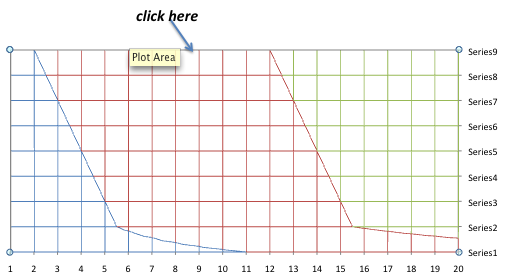
Select Format → Gridlines. In the dialog box that opens, select the Scale icon ![]() and change
the Major Unit to 0.5, the Maximum to 5.0, and the Minimum to 0.0.
and change
the Major Unit to 0.5, the Maximum to 5.0, and the Minimum to 0.0.
Equipotential Measurements
on the Point Electrodes Configuration
Replace the parallel plate electrode sheet with the two point-charge (di-pole) electrode sheet.
1. Connect the sheet to the power leads. Adjust the voltage between the two electrodes to 5.0 volts with the voltmeter and record the value in cell M30.
2. Repeat the equipotential measurements for the even-numbered 11 rows and 15 columns as carried out in the first part with the parallel plate electrodes, and record the results on the second data table on the spreadsheet.
3. Select all the data you have obtained and use the Chart Maker to make a contour plot of the potential data. Select the Gallery icon
and from the submenu tabs select the Charts ![]() button, then the Surface
button, then the Surface ![]() button. From the submenu, select the fourth icon, Wireframe Contour .
button. From the submenu, select the fourth icon, Wireframe Contour .
When the chart is plotted, select the frame by clicking the mouse on the frame of the plot itself as shown below. You will know you selected the right spot when the four corner "handles" appear.
Select Format → Gridlines. In the dialog box that opens, select the Scale icon ![]() and change
the Major Unit to 0.5, the Maximum to 5.0, and the Minimum to 0.0.
and change
the Major Unit to 0.5, the Maximum to 5.0, and the Minimum to 0.0.
4. Locate and size the Chart below the first Chart, but not beyond column R in width.
The contours of equal voltage that appear on the graph are the equipotentials of the point electrodes configuration.