PERIODIC MOTION:
OSCILLATIONS
PROCEDURE
SETTING UP THE APPARATUS
The basic set-up should have been completed for you prior to lab, but you may need to make a few adjustments before taking data. A schematic of the basic arrangement is illustrated in Figure 7-1. The oscillating mass consists of standard weights on a hanging weight carrier suspended from the end of the spring.
The motion detector "sees" the bottom of the weight carrier and reports this position to the DataLogger unit. Data collected by the DataLogger unit is sent to the serial port of the computer and displayed on the computer screen via the LoggerPro application.
2. Open the SHM-Motion link. A graph with labeled axes should appear on your computer screen.
3. Suspend the spring WITHOUT weights, large end up, from the support hook, and position the motion detector on the floor directly under the spring. Do this by sighting through the spring from above to locate the appropriate position of the detector on the floor.
5. Pull the mass straight down about 10 cm and then release it. Don't push it when you release it; just release it cleanly.
6. After setting the mass in motion, click Collect in the LoggerPro window to begin data collection. Be sure the detector "sees" the mass over its full range of motion. There should be no flat portions to your graph. If there are reposition the mass to a slightly higher point and begin again. Some sources of error could be the detector "seeing" the bench or the clamp, so try to move it as far away from these items as is feasible.
7. Adjust the distance scale in the Graph Window so that the data nearly fills the graph. To do this, double click anywhere on the graph to get a dialog box; then, under the Axis Options tab, set the necessary maximum and minimum distance values.
8. When you are satisfied with your set-up and are ready to take actual data, open the SHM Workbook and fill in the header information. Then move on to the activities below.
1. To display the graphs for distance and velocity, open the Distance-Velocity link.
2. Pull the mass straight down by about 10 cm and then release it. Don't push it when you release it; just release it cleanly.
3. After setting the mass in motion, click Collect in the LoggerPro window to begin data collection. Be sure the detector "sees" the mass over its full range of motion. There should be no flat portions on your graph. If there are, reposition the detector and begin again.
4. Adjust the vertical scale in the Velocity Graph window so that the data nearly fills the graph. To do this, double click anywhere on the graph to get a dialog box; then set the necessary maximum and minimum velocity values.
5. When you are satisfied with your graphs, COPY and PASTE them into the indicated space on the Worksheet.
1. To measure the period and frequency of the motion represented by the graph, select Examine under the ANALYZE menu in the LoggerPro window. A vertical line with a cursor will appear. Drag this line to various points on the curve. Values for the x- and y-coordinates of the graph at the position of the cursor will appear on the bottom of the screen---these are the respective time and distance and the time and velocity coordinates.
2. Set the vertical line at the left-most peak of the distance graph. Record the time listed below the graph in cell E37 of the Worksheet.
3. Move
the vertical line to the right, counting peaks as you go. Set the vertical
line on the right-most peak. Record the time given below the graph
in cell E38 of the Worksheet. Also record the number of cycles
you counted in cell E39. The total time is the difference between
these two time values. The period of the motion is the total time
divided by the number of cycles counted; that is, the period is the time
for one cycle. The frequency is the number of cycles per second, or the
reciprocal of the period.
4. Use the cursor again to determine the closest distance and the farthest distance of the oscillating mass from the detector. Enter these values in cells E45 and E46 of the Worksheet.
The equilibrium position is midway between the closest and the farthest distances. The amplitude is the difference between either the farthest distance and the equilibrium distance, or the closest distance and the equilibrium distance. The spreadsheet will do the calculation and display the result.
2. Transfer your data (in kg and meters) for both mass and position to cells B55 and C55 of the Worksheet.
3. Add a second 100 g mass (so the total is now 250 grams) and measure the equilibrium position again. Transfer these data to cells B57 and C57 of the Worksheet. Repeat with a third mass of 350 grams, and enter the data in cells B59 and C59.
The spring constant k is equal to:
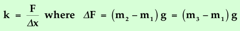
We'll call the first mass m1, and the other two masses m2 and m3, respectively.
4. The spreadsheet will automatically find the difference in force and the difference in mass, and perform the appropriate division with each pair of data points. The average value of k is displayed in cell F61.
2. Place a total of 250 grams (150 grams plus 50 gram holder) on the spring.
3. Start the mass oscillating with amplitude of about 10 cm, and record this motion on the screen. Again, make sure the curve is not "flat-topped".
4. Change the Time axis to display about three complete cycles, and adjust the Distance, Velocity and Acceleration scales until the graphs nearly fills the axes.
5. Select the combination graph and use EDIT...COPY from the LoggerPro window, and then EDIT...PASTE on the Worksheet.
6. Print out the Worksheet and use it to develop your lab report.